
Dimensional modeling is time -proven access to building data ready for analysis. While many organizations are moving to modern platforms such as databricks, these basic techniques still apply.
In Part 1 we designed a dimensional scheme. IN Part 2We built the ETL pipe for dimensions. Now, in Part 3, we implicate ETL logic for fact tables, emphasizing efficient and integrity.
Fact tables and delta extracts
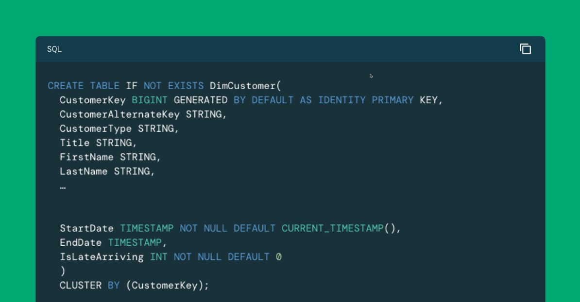
IN First blogWe have defined a table of facts FalseAs shown below. Compared to our dimensions tables, the facts table is relatively narrow in terms of recording length, with links to foreign key links to our dimensional tables, our real measures, our degenerated dimensional fields and the only metadata field present:
NOTE: We have changed in the example below Create a table Stamente From our first post that includes definitions of foreign keys instead of defining them in SepParate Change table commands. We also include primary keys to the fields of degenerated dimensions to be more expressed in this table.
The definition of the table is quite simple, but sometimes it is worth discussing LastmodifiedDatetime Field of metadata. While fact tables are relatively narrow in terms of field number, they tend to be very deep in terms of rows. Fact tables often contain millions, if not billions, records, often with high volume operating activities. Instead of attempting to reload the table with a complete extract in each ETL cycle, we usually limit our efforts to new records and those that have changed.
Depending on the source system and its basic infrastructure, there are many ways to find out which operational records must be extracted by the ETL cycle. Change data capture (CDC) Capability implemented on the operating side are the most gloomy mechanisms. But when they are not available, we often return to time stamps recorded with each transaction record because it is created and modified. This approach is not opaque for the detection of changes, but as evidenced by any experienced ETL development, it is often the best.
NOTE: Introduction LAKEFLOW CONNECT It provides an interesting option for capturing data change data in relational databases. This ability is in the preview at the time of this blog. Yet, because the ability to expand more and more RDBMSS, we expect to provide an effective and effective mechanism for increasing extracts.
In our table LastmodifiedDatetime The field captures such a time schedule recorded in the operating system. Before extracting data from our operating system, we check the facts table and identify the latest value for this field that we have seen. This value will be the starting point of our incremental (aka delta) extract.
Factual workflow ETL
A high -level workflow for our facts
- Regiment of the latest LastmodifiedDatetime Value from our facts table.
- Extract on transaction data from the source system with time stamps on the latest or after the latest LastmodifiedDatetime value.
- Do any additional steps to clean the data required on extracted data.
- To publish any values of a member of the late incoming to related dimensions.
- Search for foreign keys from associated dimensions.
- Publish data in the fact table.
In order to make digestion easier for this workflow, we describe its key phases in the following parts. Unlike the Dimension ETL post, we implement our logic for this workflow using SQL and bag combining on the basis of which language makes each step the most stragghtforward to implement. One of the strengths of the Databricks platform is again support for multiple languages. Information about the presentation as an all-oo-no option made at the peak of the alarm, we will show how data engineers can rotate quickly between them in a single implementation.
Steps 1-3: Delta extract phase
The first two steps of our workflow focus on the extraction of new and newly updated information from our operating system. In the first step we perform a simple search for the latest recorded values for LastmodifiedDatetime. If the fact table is empty because it should be after initialization, we define the default value that is far enough in time that we believe it will capture all receiving data in the source system:
Now we can use this value to extract the required data from our operating system. Although this question includes relatively details, focus your attention on the WHERE clause, where we use the last observed time stamp from the previous step to obtain individual line items that are new or modified (or associated with sales orders that are new or modified):
As previously, extracent data is persisted on the table in our staging scheme, accessible only to our data engineers, before the subsequent steps in the workflow. If we have any further data cleaning, we should do so now.
Step 4: Phase of Members of the Late Incoming Members
A typical sequence in the Warehouse ETL data cycle will start our dimension E. Organization for this method can be better ensured that all the information needed to connect our facts to dimension is introduced. However, in terms of new dimension data, narrow windows are and is picked up by a transaction record relevant. This window increases if we have a failure in the overall E. Cycle that delays the extraction of facts data. And races can always be a reference failure in the source system that allows dubious data to appear in the transaction record.
In order to insulate the Beselves from this problem, we put in the table of the dimensions of any value of the business keys found in our staged data of facts, but not in the set of current (nexposy) records for this dimension. This approach creates a record with a business (natural) key and a replacement key to which our fact table can refer. These records will be labeled as late arrival if the targeted size 2 dimension is type 2 so that we can update the appropriation on the next e-list. cycle.
In order to start, we will build a list of key business areas in our production data. Here we use strict names that allow us to dynamically identify the following fields:
NOTE: We switch to Python for the following code examples. Databricks supports the use of multiple languages, even within the same workflow. In this example, Python gives us a little greater flexibility, while still coping with the SQL concepts, which makes traditional SQL developers available.
Note that we have separated in data keys from other business keys. We will return to those for a little, but for the time being, let’s focus on no -rande (other) keys in this table.
For each commercial key without a date we can use conventions of the naming of the field and table to identify the table of dimensions that should hold this key and then make a Left-semi joint (Similar to not in () comparison, but if necessary support of conformity with multiple columns) to identify any values for this column in the staging table, but not in the dimension table. When we find an unrivaled value, we simply put it in a dimension table with the appropriate settings for Islatearriving Field:
This logic would work well for our data references if we wanted to provide records of the facts associated with valid items. However, many Downstream BI systems implement logic that requires the dimension to accommodate a continuous, uninterrupted number of data between the earliest and latest recorded values. If we support the date before or after the scope of the values in the table, we must not only enter the missing member, but to create other values needed to maintain uninterrupted scope. For this reason, we need a slightly different logic for any late arrival data:
If you did not work much with the databricks or Spark SQL, the question in the core of this last step is probably alien. Tea sequence() The function creates a sequence of values based on the specified start and stop. The result is a field that we can then explode (using Explode () Function), so each element in the field forms a line in a set of results. From there we simply compare the required ranges with what is in the dimension table to see which elements need to be inserted. With this insertion, we ensure that in this dimension is filled with a substitute key value as a Intelligent key To make our facts something that refers to.
Steps 5 – 6: Phase of Data Publication
Now that we can be sure that all business keys in our staging table can be associated with their corresponding dimensions, we can continue with the publication in the facts table.
The first step in this process is to search for foreign keys for these business keys. This can be done within a single publication step, but a large number of connections in the query often make this approach for mainaine demanding. For this reason, we could take less efficient but easier to comprehend and adjust access to searching foreign key values one business key at once and attach these values to our staging table:
Again, we use naming conventions to make this logic easier to implement. Because for the date is A dimension of playing roles Therefore, it monitors convention with more variable names, implementing slightly different logic for these business keys.
At this point, our staging table is placed in business keys and alternative key values along with our measures, degenerated fields of dimensions and Lastmodifieddate Value extracted from our source system. To make more manager, we should match the available fields with those supported by the facts table. To do this we have to drop from the business keys:
NOTE: Tea source The data frame is defined in the previous code block.
After aligning the fields, the publication step is simple. We compare our records of the inability in the table of reality based on fields of degenerated dimensions that serve as the only identifier for our facts on facts, and then update or insert values as needed:
The next steps
We hope that this blog series was for those who see that they are informative on the databricks platform. We expect a lot of experience with this data modeling approach and ETL workflows will find databricks known, accessible and capable of supporting long -established patterns with minimal change compared to what could be implemented on RDBMS platforms. If there are changes such as the ability to implement the logic of workflow using a combination of Python and SQL, we hope that data engineers consider it to implement and support their work over time.
You want to know more about databricks sql, visit our Site Now read the documentation. You can also see Tour of the product for databricks sql. Suppose you want to migrate your existing warehouse for a high -performance and server without a server with a great user experience and a lower total number of costs. In this case, the solution of the databricks SQL – the solution – is Try it free of charge.